dpl - Dalsoft's Parallel Library - is the library that consists of the routines that:

provide parallel implementation for various basic serial stencils
provide parallel implementation for conditional functions and stochastic ordering
provide parallel implementation of the Gauss–Seidel method to solve a linear system of equations
provide parallel implementation of the general 2D 5-points stencil

For the users manual of this product click here.

Here we will

provide the general description of the functions implemented
analyze the performance and accuracy of the results generated by functions from this library
show how to apply the developed technology to parallelize the code of your choice
discuss the availability of the product and port to different systems

functions/algorithms implemented by the library

dpl allows parallel execution of a number of sequential algorithms. As the supported algorithms are inherently sequential, significant mathematical transformations are necessary for their parallel implementation.

Basic Stencils

dpl offers the following functions that provide parallel implementation for the various serial stencils:

One-point stencils

dpl_stencil_1p

x[i] = b(i) + a(i)*x[i-STRIDE]

dpl_stencil_o_1p

x[i] = c(i)*x[i] + b(i) + a(i)*x[i-STRIDE]

dpl_stencil_div_1p

x[i] = b(i) + a(i)/x[i-STRIDE]

dpl_stencil_o_div_1p

x[i] = c(i)*x[i] + b(i) + a(i)/x[i-STRIDE]

Two-points stencils

dpl_stencil_2p

x[i] = a(i)*x[i-1] + b(i) + c(i)*x[i-2]

dpl_stencil_o_2p

x[i] = d(i)*x[i] + b(i) + a(i)*x[i-1] + c(i)*x[i-2]

Accumulative stencils

dpl_stencil_acc

acc = b(i) + a(i)*acc

dpl_stencil_div_acc

acc = b(i) + a(i)/acc

General stencil

dpl_stencil

x[i] = b(i) + ∑_j<ia(i,j)*x[i]

Parallel implementation of conditional functions

Plain conditional functions

dpl_stencil_min

x[i] = min( a(i)*x[i-1], b(i) )

dpl_stencil_max

x[i] = max( a(i)*x[i-1], b(i) )

Stochastic ordering

Here we provide only a brief description of the items necessary to define the implemented functions; see this for the more complete and extensive explanation.

We define vector x of the size N to be a stochastic maximum of the vectors a and b of the size N:

x = max_st( a, b )

as the solution of the following system of equations:

for every i = 0...N-1

∑( j=i...N-1:x[j] ) = max( ∑( j=i...N-1:a[j] ), ∑( j=i...N-1:b[j] ) )

dpl_max_st

x = max_st( a, b )

dpl's function dpl_stochastic_max

int dpl_stochastic_max( N, a, x )

unsigned long N,
const double *b,
double *x

)

performs parallel calculation of the output matrix x of the size NxN to be the stochastic matrix of the input matrix b of the size NxN as the following stencil:

( with m[j,*] representing j's row of the matrix m )

x[0,*] = b[0,*]
x[i,*] = max_st( x[i-1,*], b[i,*] ) for i = 1...N-1

Parallel implementation of the Gauss–Seidel method to solve a linear system of equations

dpl's function dpl_gs performs parallel execution of the Gauss-Seidel method to solve a linear system of equations ( see this for the description of the implemented Gauss-Seidel method ). The provided implementation consistently outperforms by a huge margin the serial implementation of the Gauss-Seidel method.

Parallel implementation of the general 2D 5-points stencil

dpl's function dpl_p1p0_p0p1_p0p0_p0n1_n1p0

int dpl_p1p0_p0p1_p0p0_p0n1_n1p0(

unsigned long rows, unsigned long cols,
const double *ap1p0,
const double *ap0p1,
const double *ap0p0,
const double *ap0n1,
const double *an1p0,
const double *b,
double *x

)

performs parallel execution of the general 2D 5-points stencil as following:

Implementation Note

The technology we developed allows successful parallel implementation of the great variety of serial stencils. The stencils actually parallelized ( and listed in this document ) are only a part of what can be done. Please Contact us to discuss the parallel implementation of serial stencils of your choice.
See this for more on that.

While developing dpl we discovered, studied and implemented the great variety of techniques and methods that may improve code performance, e.g. techniques for hiding memory latencies - see this for example of it use.

dpl achieves parallel implementation of supported functions by performing mathematical transformations on the underlying algorithm producing a parallel algorithm; of course, when programming this algorithm ( in C ) the care is taken of many aspects of computation such as cache utilization, load balancing, process synchronization etc.

Analysis of the performance and accuracy of the implemented functions

We performed comprehensive study of the parallel implementation of the functions from dpl analyzing the accuracy of the generated results and evaluating their performance; we compared this data to data collected while executing the corresponding serial code and/or library functions.
The following lists the results for

basic stencils : click here for results
conditional functions and stochastic ordering : click here for results
Gauss–Seidel method to solve a linear system of equations : click here for results
general 2D 5-points stencil : click here for results

While comparing timing for different kinds of code the following algorithm was used:

1 - ( timeOfTheParallelCode / timeOfTheReferenceCode )

For example if the reference code run for 8.97 seconds and the parallel code run for 3.31 seconds the improvement of 63% was reported. Note that improvement calculated in such a way never exceed 100%. Also note that improvement of 50% means that parallel code is twice as fast as the reference code, the improvement of 75% means that parallel code is four times faster that the reference code.

While studying basic stencils we just executed code on as many multi-core CPU's as we could get access to.

Studying stochastic ordering, Gauss–Seidel method to solve a linear system of equations and general 2D 5-points stencil as well as evaluating the use of the dpl library in benchmarks was much more comprehensive as we attempted to achieve many goals:

to verify accuracy of the results of the parallel code
to compare the performance of the parallel code to the performance of different implementations of the same or similar algorithms ( e.g. code from a library )
to understand how the size of the problem and/or the number of available threads affects performance

While comparing timing for different kinds of code the following algorithm was used:

The codes were executed under Linux operating system and, if not stated otherwise, the Intel(R) Xeon(R) Gold 6226R CPU @ 2.90GHz with 16 threads processor from the Microway's compute cluster was used; we are grateful for the HPC time provided by Microway, Inc..

When it was desirable to use different number of threads, that was established using the standard OpenMP/bash command sequence:

OMP_NUM_THREADS=number_of_threads;export OMP_NUM_THREADS;

Such an approach ensures that execution environments differ only by the number of threads utilized; the latency of instructions, memory access costs, sizes of caches are the same.
The threads numbers we studied are 6, 8, and 10 which corresponds to the threads numbers available on the commonly sold workstations CPU's.

Note that stencil computations are memory bound, thus stencil code efficiency is often impaired by the high memory access costs. As of now, memory access remains the weak point of the multi-core CPUs, therefore the expectations of the stencils parallel code improvements shall be reasonable.
To achieve performance gains the code that uses dpl shall be executed on a robust multi-core CPU. Running such a code on a cloud-based alternatives to physical hardware or WSL didn't show much of an improvement.

Analysis of the accuracy and performance of the implemented basic stencils

Accuracy

Because dpl implements desirable algorithms differently from the way it is done by a sequential implementation of the corresponding formula, it is necessary to verify:

How different are the results generated by parallel code from the results generated by the corresponding sequential code

Also, due to the inexact nature of the floating point calculation, the results generated by the sequential code may not be fully trusted. It is therefore necessary to verify

How different are the results generated by parallel code from the precise ( calculated with unlimited precision ) results that implement sequential algorithm

The implemented verification process is almost identical to the one described in the chapter testing dco parallelization of a stencil found here.
The results of this verification show that, in most cases, the difference between parallel and sequential results is acceptably small.
However there are exception to this - functions that use division:
dpl_stencil_div_1p, dpl_stencil_o_div_1p and dpl_stencil_div_acc.

Let study such an exception - case with the difference between the result generated by the dpl provided parallel code and the result generated by the corresponding sequential code appears to be "big".

In most cases the results to be verified are vectors of double precision values.
Define norms that will help with evaluation. For vectors x and x1 of the size ( dimension ) n we define:

Maximal Relative Difference ( MaxRelDiff )

max( fabs( 2.*( x[i] - x1[i] ) )/( fabs( x[i] ) + fabs( x1[i] ) ), i=0,...,n-1

Vector Relative Difference ( VectorRelDiff )

|x - x1|/|x1|
where
|vector| = √ ∑( vector[i] )²

Vector Normal Difference ( VectorNormDiff )

max( | x[i] - x1[i] | ), for i = 0,...,n-1

Comprehensive evaluation of the function dpl_stencil_o_div_1p using drt based evaluation procedure ( see this for more information ) reported the following data for the worst case detected:

stencil_div_o_1p cmp_parallel_serial_loop
MaxRelDiff:        3.265649e-04
VectorRelDiff:     2.630082e-04
VectorNormDiff:    1.710950e-01
Happen in the test case 3804350 at the index 875 of 1000 with the stride 1
dplRslt=-523.83780351572954714
exRslt= -524.00889851128829378
Total 7119197, Attempted 7119197, Done 7119197 cases for 1000 seconds error count = 10152.
Random number generator seed used 1596510236.

The data seems to be disappointing, the result derived by using dpl parallel library ( dplRslt ) agrees with the result generated by the sequential code ( exRslt ) in less than 4 decimal places. Also, all the norms show low level of convergence.
Let further investigate this case.
First, we create serial implementation of the function dpl_stencil_o_div_1p using the routines from the Dalsoft's High Precision ( dhp ) library ( see this for details ) - the result produced by this implementation we will call preciseRslt; we assume that the preciseRslt, generated utilizing floating point numbers with 128-bits mantissa, is fully accurate when expressed as 64-bit double precision value.
Second, taking advantage of the functionality supported by drt, we recreated the case to be studied ( establishing the used seed and skipping 3804350 cases to the case where the problem was observed ) and perform the following testing on it:

compare the result, derived by using dpl parallel library, - dplRslt - with the preciseRslt.
compare the result, generated by the sequential code, - exRslt - with the preciseRslt.

comparing the result derived by using dpl parallel library - dplRslt - with the preciseRslt, generated the following data:

stencil_div_o_1p cmp_parallel_serialhp
Dim.errs.chsums 1000 0 0 -6777.462714921427505
-6774.995656373027487
MaxRelDiff 3.925580826263917e-04
VectorRelDiff 3.161913979263145e-04
VectorNormDiff 2.055964094892033e-01

comparing the result generated by the sequential code - exRslt - with the preciseRslt, generated the following data:

stencil_div_o_1p cmp_serial_serialhp
Dim.errs.chsums 1000 0 0 -6779.515773068097587
-6774.995656373027487
MaxRelDiff 7.191229955145954e-04
VectorRelDiff 5.793222860496758e-04
VectorNormDiff 3.766914050479500e-01

The following table summarizes the above results.
Each row represents the norm being used.
The first column contains values for these norms when comparing the result derived by using dpl parallel library - dplRslt - with the preciseRslt.
The second column contains values for these norms when comparing results generated by the sequential code - exRslt - with the preciseRslt.

	dplRslt vs preciseRslt	exRslt vs preciseRslt
MaxRelDiff	3.925580826263917e-04	7.191229955145954e-04
VectorRelDiff	3.161913979263145e-04	5.793222860496758e-04
VectorNormDiff	2.055964094892033e-01	3.766914050479500e-01

While analyzing the data from this table it becomes clear that presiceRslt is closer to dplRslt than to exRslt - all the norms for dplRslt vs preciseRslt are smaller than the corresponding norms exRslt vs preciseRslt.
The problem we observed ( low precision ) seems to be due to the fact that the function dpl_stencil_o_div_1p, that performs division, is inherently unstable and thus may not be used on an arbitrary ( random-generated ) input.

Analysis of the performance of the implemented basic stencils

Reasons for the problematic performance

The goal of this project is, by using parallelization, to achieve performance gain over performance of the serial code. That is not always achievable. In this section we provide the reasons for that and offer guidelines to obtain the desirable performance gain.

Invoking and executing parallel code causes significant performance penalties:

invoking parallel code is very expensive, routines that start and maintain a parallel region are complicated and take significant time to execute
the created ( by dpl ) parallel code is the result of a significant mathematical transformation to the original code, it performs more operations ( hopefully in parallel ) than the original sequential code

In order to achieve performance gains ( in spite of the above described performance penalties ) the supported functions are executed in parallel mode only if certain conditions are met. These conditions depend on the size of the problem ( number of elements to be processed ) and characteristics of CPU that will execute the parallel code ( e.g. number of threads available ). The restrictions listed bellow are not exact and in certain cases may not suffice to achieve performance gains.

The following table establishes condition for the dpl implemented parallel code to be faster than the corresponding serial code: for every implemented function the minimal size of the problem ( number of elements to be processed ) is listed for the number of threads available. Note that the affect of the STRIDE parameter on the execution time of the parallel code may be detrimental, the values listed in table are for STRIDE being equal to 1.
Each row represents the basic stencil provided by dpl. Each column lists the number of threads available. The value in the table is the minimal size of the problem ( number of elements to be processed ) for the parallel code to be faster than the corresponding sequential code - dpl checks for these conditions and, if they are not fulfilled, the parallel executions is aborted and an error is returned.

	2	3	4	5	> 5
dpl_stencil_1p x[i] = b(i) + a(i)*x[i-1]	850	1000	900	900	1125
dpl_stencil_o_1p x[i] = c(i)x[i] + b(i) + a(i)x[i-1]	1250	1250	900	900	950
dpl_stencil_div_1p x[i] = b(i) + a(i)*x[i-1]	750	600	500	600	600
dpl_stencil_o_div_1p x[i] = c(i)*x[i] + b(i) + a(i)/x[i-1]	650	600	500	500	650
dpl_stencil_acc acc = b(i) + a(i)*acc	1250	1125	1250	1250	1450
dpl_stencil_div_acc acc = b(i) + a(i)/acc	300	400	450	450	550
dpl_stencil_2p x[i] = a(i)x[i-1] + b(i) + c(i)x[i-2]	⁽¹⁾	4000	2500	1750	2250
dpl_stencil_o_2p x[i] = d(i)x[i] + b(i) + a(i)x[i-1] + c(i)*x[i-2]	⁽¹⁾	2000	1000	1250	1000
dpl_stencil x[i] = b(i) + ∑_j<ia(i,j)*x[i]	150	175	200	200	250

(1) for the specified number of cores the dpl generated parallel code will be always slower than the corresponding serial code

Timing

The following table presents results of comparison of the execution time achieved by the parallel version over the execution time achieved by the sequential version of the same algorithm.
Each row represents the the basic stencil provided by dpl. Each column lists the CPU used in comparison. The value in the table is the improvement of the execution time of the parallel code over the execution time of the sequential code achieved on the specified CPU - see this for the explanation on how these values were calculated.

All codes were executed under Linux operating system on four different CPU's:

vintage: Intel(R) Core(TM) Duo E8600 @ 3.33GHz CPU with 2 threads
mainstream: Intel(R) Core(TM) i5-9400 @ 2.90GHz CPU with 6 threads
advanced: Intel(R) Xeon(R) Silver 4110 CPU @ 2.10GHz with 16 threads
extreme: Intel(R) Xeon(R) Gold 6226R CPU @ 2.90GHz with 16 threads

It was attempted to run the code under the same conditions on the system with the minimal possible load. Every code segment was executed 3 times with the execution time used for calculation of the improvement being neither the best nor the worst.

The size of the problem ( number of elements to be processed ) was set to 10000 for all the functions except dpl_stencil - for this function the size of the problem ( number of elements to be processed ) was set to 1000.
The same arguments were used when executing sequential and parallel codes. The arguments were a double precision random numbers in the range [-1.5;1.5] generated using Dalsoft's Random Testing ( drt ) package - see this for more information.

	Core(TM) Duo E8600	Core(TM) i5-9400	Xeon(R) Silver 4110⁽¹⁾	Xeon(R) Gold 6226R⁽¹⁾
dpl_stencil_1p x[i] = b(i) + a(i)*x[i-1]	54%	51%	71%	73%
dpl_stencil_o_1p x[i] = c(i)x[i] + b(i) + a(i)x[i-1]	30%	47%	58%	74%
dpl_stencil_div_1p x[i] = b(i) + a(i)*x[i-1]	23%	58%	76%	82%
dpl_stencil_o_div_1p x[i] = c(i)*x[i] + b(i) + a(i)/x[i-1]	24%	52%	69%	83%
dpl_stencil_acc acc = b(i) + a(i)*acc	26%	53%	72%	71%
dpl_stencil_div_acc acc = b(i) + a(i)/acc	64%	68%	84%	86%
dpl_stencil_2p x[i] = a(i)x[i-1] + b(i) + c(i)x[i-2]	⁽²⁾	41%	66%	72%
dpl_stencil_o_2p x[i] = d(i)x[i] + b(i) + a(i)x[i-1] + c(i)*x[i-2]	⁽²⁾	41%	66%	72%
dpl_stencil x[i] = b(i) + ∑_j<ia(i,j)*x[i]	43%	73%	63%	60%

(1) the benchmarks were executed on Microway's compute cluster; we are grateful for the HPC time provided by Microway, Inc.
(2) dpl generated parallel code will be always slower than the corresponding serial code

Analysis of the parallel implementation of conditional functions

Analysis of the parallel implementation of the plain conditional functions

Accuracy

The results of this verification show that, on the same inputs, the differences between dpl_stencil_min and dpl_stencil_max generated results and results generated by the serial implementation of the corresponding function are acceptably small.

Timing

The algorithm used by dpl to implement plain conditional functions is very complicated and execution time that takes to execute parallel functions dpl_stencil_min and dpl_stencil_max depends on the values of the a vector and, to a lesser extend, on the values of the b vector.
The following table presents improvement of the parallel function dpl_stencil_max over the serial version of the same function. Each column represents the number of elements being used; the vectors a and b consist of randomly generated double precision values; generation of random values was done using Dalsoft's Random Testing ( drt ) package - see this for more information.

	10000	100000	1000000
parallel/serial	54%	84%	88%

However there are distributions of a and b processing which produce less spectacular improvements, although no case when serial implementation is faster that the corresponding parallel version, was observed.

Analysis of the parallel implementation of the stochastic ordering

Accuracy

The results of this verification show that, on the same inputs, the differences between dpl_stencil_max_st and dpl_stochastic_max generated results and the results generated by the serial implementation of the corresponding algorithm are acceptably small.

Timing

The following table presents improvement of the parallel function dpl_stencil_max_st over the serial version of the same function. Each column represents the number of elements being used; the vectors a and b consist of double precision values generated using Dalsoft's Random Testing ( drt ) package - see this for more information.

	10000	100000	1000000
parallel/serial	56%	63%	54%

The following table presents improvement of the parallel function dpl_stochastic_max over other implementations of the underlying algorithm, namely:

"quick parallel" implementation
the desirable stencil x[i,*] = max_st( x[i-1,*], b[i,*] ) is implemented as
dpl_max_st( N, x[i-1.,*], b[i,*], x[i,*] )
note that "quick parallel" implementation of the underlying algorithm is not part of the dpl library
serial implementation
call to the serial function dpl_stochastic_max_serial
Parallel Vincent's Algorithm
the mainstream parallel implementation of the underlying algorithm; it is called "Parallel Vincent's Algorithm", see this for more information. Also see this for additional evaluation data.
The parallel implementation of the Vincent's algorithm used in this study was created by utilizing OpenMP.

Every column represents the number of rows being used in the the input matrix that consists of the double precision values generated using Dalsoft's Random Testing ( drt ) package - see this for more information. The double precision values generated in such a way that makes input matrix to be a transition probabilities matrix in a Markov chain.
Each row lists the improvements of the the parallel function dpl_stochastic_max over other implementations of the underlying algorithm.

	1000	5000	10000	20000	30000	40000	50000	60000	70000
parallel/quick parallel	76%	65%	56%	40%	30%	24%	20%	22%	21%
parallel/serial	20%	75%	79%	77%	73%	70%	66%	63%	60%
parallel/parallel Vincent	-170%	20%	40%	65%	53%	55%	53%	50%	50%

From the above data some interesting conclusions may be derived:

the parallel function dpl_stochastic_max is always faster than corresponding serial implementation of the underlying algorithm
the parallel function dpl_stochastic_max is always faster than quick parallel implementation of the underlying algorithm
the parallel function dpl_stochastic_max is faster than parallel Vincent's implementation, except for the small input matrices
quick parallel implementation of the underlying algorithm is faster than corresponding serial implementation, except for the small input matrices
for reasonably large input matrices the quick parallel implementation of the underlying algorithm is faster than parallel Vincent's implementation

Analysis of the the parallel implementation of the Gauss–Seidel method to solve a linear system of equations

The following are the results of comparison of the dpl_gs function with the

serial implementation of the Gauss-Seidel method to solve a linear system of equations
function LAPACKE_dgesv from LAPACK under OpenBLAS using LAPACKE C Interface ( to LAPACK )

For every case in this study the arguments used were a double precision random numbers generated using Dalsoft's Random Testing ( drt ) package ( see this for more information ) and a Strictly Diagonally Dominant Matrix was created using the described random numbers generator.

See this for the standalone version of the following study.

Comparison of the performance and accuracy for the parallel implementation of the Gauss–Seidel to the serial implementation of the Gauss-Seidel method to solve a linear system of equations

Accuracy

The results of this verification show that, on the same inputs, the differences between dpl_gs generated results and results generated by the serial implementation of the Gauss-Seidel method to solve a linear system of equations are acceptably small.

Timing

The following graph presents results of the performance comparison between parallel and serial implementations of the Gauss-Seidel method to solve a linear system of equations:

The X axis lists different sizes for the problem we attempted to study, e.g. 2000 means that the input matrix was 2000x2000 and the input/output vectors were of the size 2000
The Y axis lists percent of improvement achieved by the parallel code over the serial one; the results were calculated as described here
The legend specifies on what CPU the plotted data was generated

Comparison of the performance and accuracy for the parallel implementation of the Gauss–Seidel to solve a linear system of equations to the performance and accuracy of the library routine that solves a linear system of equations

Here we compare the dpl_gs function from the dpl library to the function LAPACKE_dgesv from LAPACK under OpenBLAS using LAPACKE C Interface ( to LAPACK ).
Both these functions solve linear equations Ax=b, where

A is the input matrix
b is the input right-hand vector
x is solution of the linear equations Ax=b

Every call to dpl_gs solves one linear equation, specified by the input arguments, utilizing threads available.
LAPACKE_dgesv allows for a given matrix to solve many linear equations by using different right-hand vectors - the input matrix is transformed into optimal representation and every linear equation is solved "quickly" using this optimal matrix(es).
For the comparison to be fair ( especially when monitoring execution time ) we utilize the following procedure:

peek up a number nrh of right-hand vectors to process
generate nrh vectors
run nrh iterations performing dpl_gs for every right hand vector generated
perform LAPACKE_dgesv for all right hand vector generated

Accuracy

The results of this verification show that, on the same input, the differences between dpl_gs generated results and LAPACKE_dgesv generated results are acceptably small.

Timing

The execution time of processing nrh cases by dpl_gs, that is reported by our test suite, is equal to:

T_total = T_setup + nrh*T_gs

where

T_setup is the time to setup the package ( random number generation etc. )
T_gs is the time that it takes to execute one invocation of the dpl_gs, doesn't depend on nrh

We assume that the execution time of processing nrh cases by LAPACKE_dgesv, that is reported by our test suite, is equal to:

T_total = T_setup + T_{dgesv_preprocess} + nrh*T_dgesv

where

T_setup is the time to setup the package ( random number generation etc. ), identical to the setup time while executing dpl_gs
T_{dgesv_preprocess} is the time that it takes to transform the input matrix into optimal representation, doesn't depend on nrh
T_dgesv is the time that it takes to process one equations using an optimal representation of the matrix, doesn't depend on nrh

Under such assumptions, provided that T_gs > T_dgesv, for any size of the matrix there is nrh such that solving nrh equations by LAPACKE_dgesv will be faster than solving the same nrh equations by dpl_gs.
Here we will calculate the even-point nrhEven of cases when, for a given size, the execution times of processing nrhEven cases by dpl_gs and LAPACKE_dgesv are the same.
For every size of the problem we studied the following procedure was utilized:

peek up reasonably large number of equations nrh to be solved - 100 in this study
run the benchmark without executing dpl_gs nor LAPACKE_dgesv - the execution time reported will be equal to T_{setup_nrh}
run the benchmark executing dpl_gs - the execution time reported will be equal to T_{total_nrh_gs} = T_{setup_nrh} + nrh*T_gs
run the benchmark executing LAPACKE_dgesv - the execution time reported will be equal to T_{total_nrh_dgesv} = T_{setup_nrh} + T_{dgesv_preprocess} + nrh*T_dgesv
double the number of equations and run the benchmark without executing dpl_gs nor LAPACKE_dgesv - the execution time reported will be equal to T_{setup_2*nrh}
double the number of equations and run the benchmark LAPACKE_dgesv - the execution time reported will be equal to T_{total_2*nrh_dgesv} = T_{setup_2*nrh} + T_{dgesv_preprocess} + 2*nrh*T_dgesv

To summarize, after applying the above procedure, we calculated:

T_{setup_nrh}
T_{total_nrh_gs} = T_{setup_nrh} + nrh*T_gs
T_{total_nrh_dgesv} = T_{setup_nrh} + T_{dgesv_preprocess} + nrh*T_dgesv
T_{setup_2*nrh}
T_{total_2*nrh_dgesv} = T_{setup_2*nrh} + T_{dgesv_preprocess} + 2*nrh*T_dgesv

and we looking for nrhEven such that

nrhEven*T_gs = T_{dgesv_preprocess} + nrhEven*T_dgesv

which can be obtained as following

T_gs = ( T_{total_nrh_gs} - T_{setup_nrh} )/nrh
T_dgesv = ( ( T_{total_2*nrh_dgesv} - T_{setup_2*nrh} ) - ( T_{total_nrh_dgesv} - T_{setup_nrh} ) )/nrh
T_{dgesv_preprosess} = ( ( T_{total_nrh_dgesv} - T_{setup_nrh} ) - ( T_{total_2*nrh_dgesv} - T_{setup_2*nrh} ) + ( T_{total_nrh_dgesv} - T_{setup_nrh} )
nrhEven=T_{dgesv_preprocess}/(T_gs-T_dgesv)

and, finally,

nrhEven=nrh*(2*(T_{total_nrh_dgesv} - T_{setup_nrh} ) - ( T_{total_2*nrh_dgesv} - T_{setup_2*nrh} ) )/( (T_{total_nrh_gs} - T_{setup_nrh}) - ( T_{total_2*nrh_dgesv} - T_{setup_2*nrh} ) + ( T_{total_nrh_dgesv} - T_{setup_nrh} ) )

The following graph shows the even points for the number of right-hand vectors being processed ( nrh ) when, for a given size, the execution times of processing nrh cases by dpl_gs and LAPACKE_dgesv are the same. Therefore if it is necessary, for a given matrix size, to solve more than that number of equations, LAPACKE_dgesv will be faster, otherwise dpl_gs will be faster.

The X axis lists different sizes for the problem we attempted to study, e.g. 2000 means that the input matrix was 2000x2000 and the input/output vectors were of the size 2000
The Y axis lists the value of an even point for a given size of the problem
The legend specifies on what CPU the plotted data was generated

Analysis of the the parallel implementation of the general 2D 5-points stencil

The following are the results of the comparison of the dpl_p1p0_p0p1_p0p0_p0n1_n1p0 function with the serial implementation of this function.

Accuracy

The results of this verification show that, on the same inputs, the differences between dpl_p1p0_p0p1_p0p0_p0n1_n1p0 generated results and results generated by the serial implementation of this algorithm are acceptably small.

Timing

The following graph presents results of the performance comparison between parallel and serial implementations of the general 2D 5-points stencil:

The X axis lists different sizes for the problem we attempted to study, e.g. 2000 means that the input input/output matrices were of the size 2000x2000
The Y axis lists percent of improvement achieved by the parallel code over the serial one; the results were calculated as described here
The legend specifies on what CPU the plotted data was generated

As can be noticed from that graph, the performance gain begin to deteriorate as the size of the problems increases - somewhere approaching 5000. We run the comparison for even larger number of elements and the problem only got worse.
The following table summarizes these results.
Each row represents the number of elements being used.
Each column represents the number of threads being utilized.

	6	8	10	16
20000	22.38%	24.07%	24.72%	25.49%
30000	6.81%	7.52%	7.63%	8.17%
40000	7.04%	7.75%	7.89%	8.29%

The code is reading from 7 input arrays and at some point, it seems to us, the CPU is not capable to keep up. To verify this presumption we created a simplified version of the 2D 5-points stencil ( actually, very useful one )
and implemented it using dpl_p1p0_p0p1_p0p0_p0n1_n1p0 routine from the dpl library. The newly created routine, as implemented, is reading from 4 input arrays ( compared to 7 input array of the original code ).
The following graph presents results of the performance comparison between parallel and serial implementations of the simplified 2D 5-points stencil:

From that graph it is clear that newly created routine holds it ground better that the original one.
Even when we run the task for larger number of elements the problem was not so profound - the following table summarizes these results.
Each row represents the number of elements being used.
Each column represents the number of threads being available.

	6	8	10	16
20000	43.08%	49.97%	52.41%	54.7%
30000	36.64%	43.29%	45.71%	47.85%
40000	30.15%	37.15%	39.21%	41.18%

applying the developed technology

Here we show

how to apply routines from the dpl in order to optimize benchmarks and/or applications
how to modify the existing code in order to utilize the technology that dpl relys on

The following contains

samples of serial code being optimized by applying our technology: see this, this and this
samples of parallel code being improved by applying our technology: see this and this

It is important to note that we don't know about any existing way to improve the code shown. The use of dpl seems to be the only currently available option to achieve that.
Please note that routines shown here are not part of the dpl package. Please Contact us to discuss the parallel implementation of a serial code of your choice.

using dpl library in benchmarks and/or applications

The following shows the results of applying routines from the dpl in order to optimize benchmarks and/or applications.

See this for the text version of the following material.

Polybench

Here we study a benchmark from the PolyBench benchmark suite - see this for information about this benchmark suite: disclaimer, copyright and how to download.

adi

We used the following code segment from the adi benchmark of the PolyBench benchmark suite:
The code was slightly modified to allow use of the routines from the dpl library.
The following graph presents results of the performance comparison between modified and the original codes.

The X axis lists different sizes for the problem we attempted to study ( the value of _PB_N )
The Y axis lists percent of improvement achieved by the modified code that uses dpl library over the original serial one; the reported results were calculated as described here
The legend specifies on what CPU the plotted data was generated

utilizing the developed technology

Here we show how the technology, developed in dpl, may help to parallelize applications that do not appear as stencils. Please Contact us to discuss the parallel implementation of a serial code of your choice.

DSP filters

DSP filters seems to be well suited for parallelization using our technology.

latnrm

We downloaded the code for the ORDER order Normalized Lattice filter processing NPOINTS points ( latnrm ) from the internet - we will refer to this code as serial version of the function:
As it appears above, it is difficult to see any code patterns ( stencils ) that might allow to apply our technology. However the code may be rewritten as ( only loops are shown )
which makes it possible for a number of the available techniques to be applied. Note that in this case none of the routines from the dpl library may be used directly. However the technology developed for the implementation of this library may be used here.

We parallelized the one-point stencil

left = Coefficients[j-1] * left - Coefficients[j] * InternalState[j]

overlapping the generated parallel code with the rest of the routine. This led to the generation of the parallel code for the latnrm DSP filter listed above.

The evaluation of the created parallel code was done under Linux operating system running on the AMD EPYC 7713 Processor with 16 threads. The following graph presents improvement of the created parallel implementation of the function latnrm over it serial version.

The X axis lists different sizes for the problem we attempted to study ( the value of NPOINTS; ORDER was always set to NPOINTS>>1; the input arrays consist of randomly generated double precision values; generation of random values was done using Dalsoft's Random Testing ( drt ) package - see this for more information ).
The Y axis lists percent of improvement ( or otherwise ) achieved by the created parallel implementation of the function latnrm over it serial version; the reported results were calculated as described here
The legend specifies on what CPU the plotted data was generated

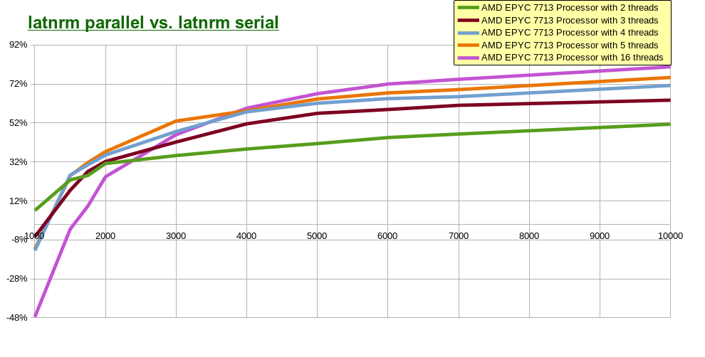
Note that change between execution time of the created parallel implementation of the function latnrm and it serial version depends on the size of the problem ( the value of NPOINTS ) as well as the number of threads utilized. Using more threads doesn't always result in faster execution time:

using 16 threads leads for fastest execution time only if the value of NPOINTS is 4000 or greater.
for smaller values of NPOINTS ( e.g. 1000 ), the best results achieved with the smaller number of threads utilized ( e.g. 2 threads for NPOINTS being 1000 ).

See this for similar study.

Computational ( quantitative ) finance

Analyzing the code samples used in computational finance, it is quite obvious about abound opportunities for parallelization. We will analyze some of it and show how the technology, developed in dpl, may be applied to improve the performance of these applications through parallelization. See this for the standalone version of the following study.

The following contains parallel implementation for the

Leisen-Reimer binomial tree: European Call and American Call
Crank-Nicolson finite difference method for option pricing: European Put
Heston stochastic volatility model: European Call

Please note that routines shown here are not part of the dpl package. Please Contact us to discuss the parallel implementation of a serial code of your choice.

Leisen-Reimer binomial tree

We use the following C++ code, developed by Dr. Fabrice Douglas Rouah ( see this ), as the base for our study.
The following optimizes European and American Call options. The corresponding Put options can be handled similarly.

Leisen-Reimer binomial tree, European Call

The European Call option is implemented by the following code portion of the original code
with n being number of time steps utilized.
We will refer to the executable derived from this code as serial implementation.
The internal loop of the above code is parallel and may be easily parallelized using OpenMP - we will refer to the executable derived from that parallel version of code as quick_parallel implementation.
However there is a way to create a better parallel code.
Perform Loop interchange of the above code getting the loop
Now the internal loop is not parallel but it is a stencil ( reminiscent to the one-point stencil dpl_stencil_1p ) and the technology, developed in dpl, may be applied to parallelize and improve this code.
The major sources of optimization of the loop after interchange are:

cache friendly memory access
one parallel invocation for all the code
the ability to create loop pipeline for the encompassing for ( i = n - 1; i >= 0; i-- ) loop

Combined with the careful coding we obtain an executable which is refereed as parallel implementation.

The following timing improvement was observed on the Intel® Core(TM) i5-9400 Processor with 6 threads.
Each column represents the number of time steps utilized. Each row represents improvement of the code of the first specified executable type over the code of the second executable type.

	1001	1501	2001	2501	3001	3501	4001	10001
parallel/quick_parallel	44.79%	39.68%	44%	41.03%	29.17%	25.71%	20.41%	11.24%
parallel/serial	-113%	-18.75%	50.88%	59.65%	58.54%	61.19%	61.76%	59.42%
quick_parallel/serial	-272%	-97%	12.28%	31.58%	41.46%	47.76%	51.96%	54.28%

From the above data some interesting conclusions may be derived:

parallel implementation is always faster that corresponding quick_parallel implementation of the underlying algorithm
for reasonably large number of time steps utilized, parallel and quick_parallel implementations are faster that serial implementation of the underlying algorithm

Leisen-Reimer binomial tree, American Call

The American Call option is implemented by the following code portion of the original code
with n being the number of time steps utilized and S being the input binomial tree.
We will refer to the executable derived from this code as serial implementation.
The internal loop of the above code is parallel and may be easily parallelized using OpenMP - we will refer to the executable derived from that parallel version of code as quick_parallel implementation.
However we will create a better parallel code.
Perform Loop interchange of the above code getting the loop
Now the internal loop is not parallel but it is reminiscent of the conditional stencil dpl_stencil_max and the technology, utilized by dpl for implementation of this stencil, may be applied to achieve the better performance for Leisen-Reimer implementation of the American Call option.
The major sources of optimization of the loop after interchange are:

cache friendly memory access
one parallel invocation for all the code
the ability to create loop pipeline for the encompassing for ( i = n - 1; i >= 0; i-- ) loop

	1001	1501	2001	2501	3001	3501	4001	10001
parallel/quick_parallel	36.79%	40.8%	42%	38.79%	32.25%	26.27%	25.45%	18.29%
parallel/serial	41.23%	69.17%	73.48%	74.64%	74.56%	73.64%	73.23%	69.54%
quick_parallel/serial	7.02	47.92	54.27%	58.57%	62.44%	64.44%	64.09%	62.73%

From the above data some interesting conclusions may be derived:

parallel implementation is always faster that corresponding quick_parallel implementation of the underlying algorithm
parallel and quick_parallel implementations are always faster that serial implementation of the underlying algorithm

Crank-Nicolson finite difference method for option pricing

Here we will use Crank-Nicolson Finite Difference Method for Option Pricing to find the numeric solution to the Black, Scholes and Merton partial differential equation ( see this for the description )

the Black–Scholes-Meron equation - a partial differential equation governing the price evolution of a European Call or European Put under the Black–Scholes model.

Where:

t - a time in years; t = 0 being initial time ( "now" )
S(t) - the price of the underlying asset at time t
V(S,t) - the price of the option as a function of the underlying asset S at time t
r - the the annualized risk-free interest rate
σ - the volatility of the stock

We assume the time is running from "now" ( 0 ) to some specified value YearsToMaturity and the price of underlying asset is running from 0 to some specified value MaxPrice.

Divide the (t,S) plane into a grid of N+1xM+1 equaly spaced points

t_i = Δt i, i = 0,...,N
S_j = ΔS j, j = 0,...,M

where Δt = YearsToMaturity/N, ΔS = MaxPrice/M.

We denote the value of the derivative at time t_i when the underlying asset has value S_j as

V_i,j = V( iΔt, jΔS ) = V( t_i,S_j ) for i = 0,...,N; j = 0,...,M

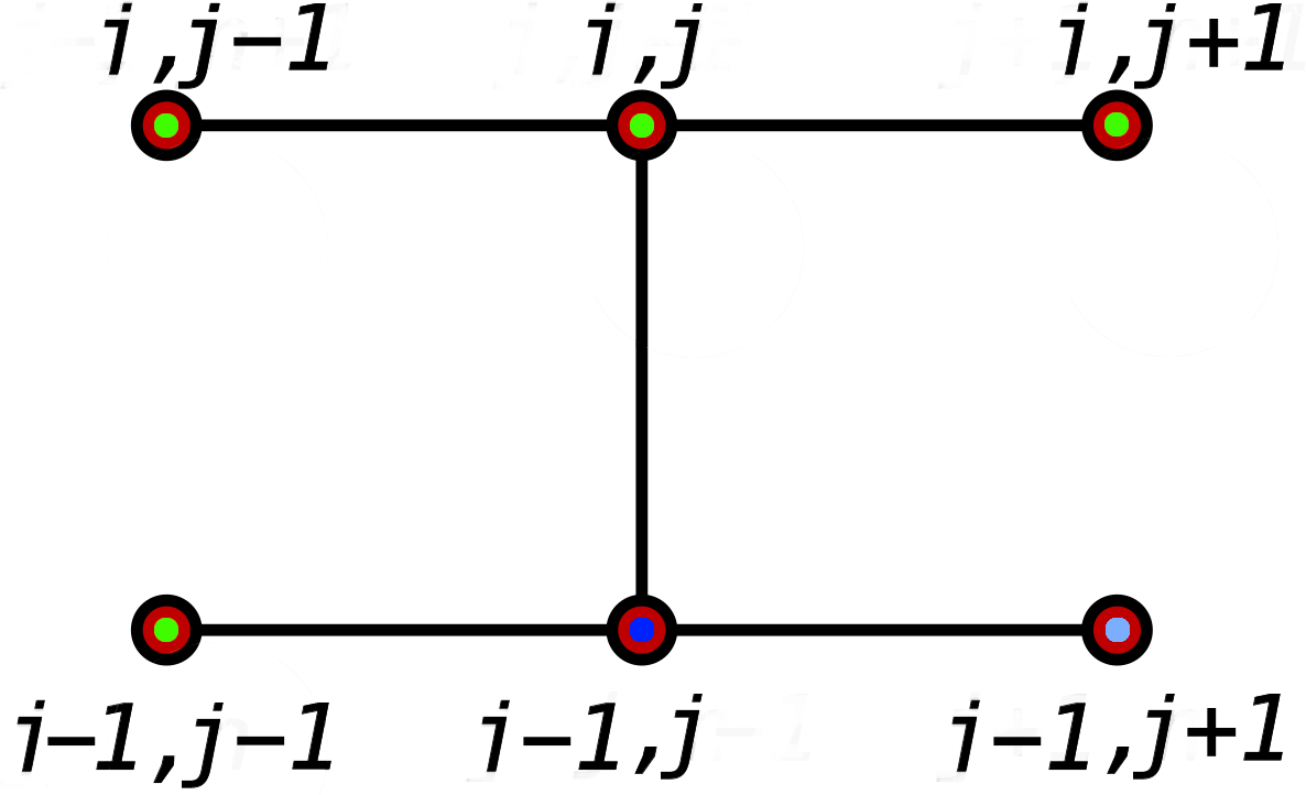
Crank-Nicolson method uses the following discretization of the above the Black, Scholes and Merton partial differential equation

−a_jV_i−1,j−1 + ( 1 − b_j )V_i−1,j − c_jV_i−1,j+1 = a_jV_i,j−1 + ( 1 + b_j )V_i,j + c_jV_i,j+1
for i = 1,...,N; j = 1,...,M-1

where

a_j = Δt( σ²j² - rj )*0.25
b_j = -Δt( σ²j² + r )*0.5
c_j = Δt( σ²j² + rj )*0.25

For a given StrikePrice, to calculate European Put option, we establish the following boundary conditions:

V_i,0 = StrikePrice*exp( ^-r(N-i)Δt) for i = 0,1,...,N
V_i,M = 0 for i = 0,1,...,N
V_N,j = max( StrikePrice - j*ΔS, 0 ) for j = 0,1,...,M

The discretization cited earlier can be rewritten as:

( 1 − b_j )V_i−1,j = a_jV_i−1,j−1 + c_jV_i−1,j+1 + a_jV_i,j−1 + ( 1 + b_j )V_i,j + c_jV_i,j+1
for i = 1,...,N; j = 1,...,M-1

V_i−1,j = A_jV_i−1,j−1 + B_j
for i = N,...,1; j = 1,...,M-1

where

A_j = a_j/( 1 − b_j )
B_j = ( c_jV_i−1,j+1 + a_jV_i,j−1 + ( 1 + b_j )V_i,j + c_jV_i,j+1 )/( 1 − b_j )

The newly created expression is a stencil for which the technology provided by dpl enables parallel execution.

Crank-Nicolson stencil

We execute these stencils for i starting with N till 1. At every given step

V_i−1,j−1 is defined by the established boundary condition ( for j being 1 ) or calculated at the previous step of the stencil ( for other values of j )
V_i−1,j+1 is defined only for j being M-1 ( as the established boundary condition ); for other values of j the currently existing value of V_i−1,j+1 is used; that requires the initialization of all the elements of V ( except the boundary described earlier ) to some reasonable initial values and iterations of the algorithm till the desirable precision has been reached
V_i,j−1, V_i,j, V_i,j+1 are defined by the the established boundary conditions ( for i being N ) or calculated at the previous iterations of the proposed algorithm ( for other values of i )

The following timing improvement was observed on the Intel® Core(TM) i5-9400 Processor with 6 threads.
We used the square grid - N being equal to M. Each column represents the value of N - number of time steps utilized. The row represents improvement of the parallel version of the described algorithm over it serial version.

	200	250	300	350	400	450	500
parallel/serial	-6.14%	17.75%	28%	37%	41%	50%	54%

Heston stochastic volatility model

Heston stochastic volatility model is an extension of the Black Scholes model that doesn't assume a volatility to be constant.

The following shows the results of optimization ( parallelization ) for calculation of a European Call option using Heston model for a discretisation technique known as "Full Truncation Euler Discretisation, coupled with Monte Carlo simulation", see this for the theoretical reference.
The implemented algorithm is as follows:

Generation of correlated normally distributed random numbers sequences
We set SpotNormalRandom array to a sequence of standard normal random numbers and set VolatilityNormalRandom to a sequence of standard normal random numbers correlated with SpotNormalRandom
to generate a sequence of standard normal random numbers:
- we first generated a sequence of pairs of an uncorrelated random variables in the range ]0.,1.[ using random number generator provided by the Dalsoft's Random Testing ( drt ) package ( see this for more information )
- then, for every pair of the generated random numbers, we applied the Box–Muller transform generating pairs of independent, standard, normally distributed random numbers - see this for explanation.

VolatilityNormalRandom

SpotNormalRandom

here

this

The generation of correlated normally distributed random numbers sequences was fully parallelized.

Calculation of the volatility price VolatilityPrices values from the VolatilityNormalRandom vector generated in the previous step

where
κ - mean-reversion rate
θ - long run average volatility
ξ - the volatility of the volatility
Δt - time derivative discretisation

We failed to parallelize the calculation of volatility prices. However, the above code was greatly optimized by applying the optimization technology utilized by the dpl, e.g. techniques for hiding memory latencies.
Calculation of the spot price SpotPrices values from the SpotNormalRandom and VolatilityPrices vectors generated in the previous steps

where
r - risk-free rate
Δt - time derivative discretization

The above code is a stencil supported by dpl and was fully parallelized.

The following timing improvement was observed on the Intel® Core(TM) i5-9400 Processor with 6 threads.
We run every simulation for 100000 iterations. Each column represents the value of NumberOfPoints - number of time steps utilized. The row represents improvement of the optimized ( parallel ) version of the described algorithm over it serial version.

	500	1000	1500	2000	2500	3000	3500
parallel/serial	61.79%	65.11%	66.68%	66.87%	66.91%	67.73%	68.54%

Parallel Polynomial Evaluation

Polynomial evaluation is a well studied topic. Many of the algorithms developed allow parallel implementation using routines provided by the dpl.

The following shows how to create parallel implementation for the Horner's method - one of the better known ways for efficient evaluation of polynomials.
Similar parallel implementation may be derived for other functions related to the Horner's method, e.g. polynomial division.

Parallelization of the Horner's method for polynomial evaluation

Horner's method for polynomial evaluation - see this for the description/explanation - represents the polynomial to be evaluated

p(x) = c₀ + c₁x + c₂x² +...+ c_nxⁿ

p(x) = c₀ + x ( c₁ + x ( c₂ +...+ x ( c_n-1 + c_nx )...))

Note, that for a and b being ( allocated ) arrays of n double precision values and set as following:

a[i] = x
b[i] = c_n-i-1
for i = 0,...,n-1

and acc being a double precision variable set as following:

acc = c_n

Horner's representation of the polynomial p(x) may be regarded as the stencil

acc = a[i]*acc + b[i] for i = 0,...,n-1

which is implemented by the function dpl_stencil_acc from dpl.
The more efficient implementation may be created utilizing the fact that all the elements of the array a have the same value.

the availability of the product and port to different systems

The current OpenMP version of dpl is available on x86 Linux systems and Windows. The OpenCL version, that supposed to run on a wide range of hardware, is also available.

Code, being written in C, can be directly ported to any sane multi-core architecture running under a system that provides a decent C compiler with OpenMP support. Please contact us if you are interested to port dpl to your system.

OpenCL version

We created the OpenCL version of the product - dpl_ocl - a while ago but due to the bug in the llvm tool chain ( see this ) could not release it. With the availability of the release 13.0 of the clang, it became possible to use llvm-spirv to create binary version of the dpl_ocl's kernels, albeit under severe restrictions: compiler optimization may not be used ( see this for details ). Not being able to optimize the product that supposed to be fast doesnt make much sense. Because of this we decided to

release the OpenCL implementation for a reasonable subset of the functions implemented by dpl - see the apropriate section in the users manual for the description and instructions on how to use.
tag this OpenCL version of the product as "experimental" and offer it free of charge - visit this for the description and download.